Visualization
rddac.plot_scan, rddac.plot_point_cloud, rddac.plot_force, and rddac.plot_traverse accept numpy arrays. Pair them with rddac.open_h5 to read the arrays from a single experiment and render them. rddac.scan_to_pointcloud bridges the two worlds: it converts a raw flat scan buffer into an (N, 3) point cloud that plot_point_cloud (and any point-cloud ML pipeline) understands.
The companion notebook at notebooks/04_visualization.ipynb reproduces every cell below.
import matplotlib.pyplot as plt
import numpy as np
import rddac

from pathlib import Path
DATA_DIR = Path('./data')      # repository root
# DATA_DIR = Path('../data')   # uncomment instead when running from inside notebooks/
experiment_id = 0              # bundled with `rddac download --small`
1. Scan image (height)
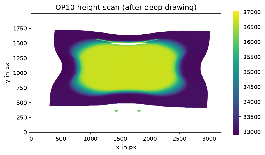
The raw laser scans are flat (6400000,) buffers stored row-major over a 2000 x 3200 pixel grid (see HDF5 structure). plot_scan reshapes the buffer and renders it as a 2D image. Two defaults do the heavy lifting:
mask_zero=True: the scanner writes0where it measured nothing; masking renders those pixels transparent so the part silhouette stands out.- The grid dimensions default to the group attrs (
x_shape=3200,y_shape=2000); pass them explicitly if you sliced the buffer yourself.
Values are raw sensor units — the mm calibration belongs to the planned preprocessing step (package v1.1).
with rddac.open_h5(experiment_id, data_dir=DATA_DIR) as f:
    z10 = f['pointcloud/op10/z'][:]
    z20 = f['pointcloud/op20/z'][:]

ax, cbar = rddac.plot_scan(z10, title='OP10 - after deep drawing')
plt.show()
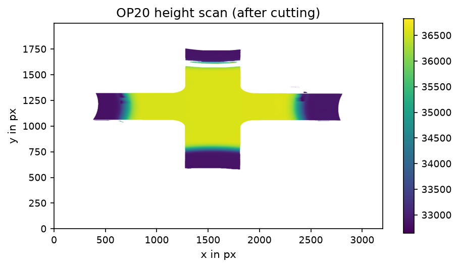
The OP20 scan shows the same part after cutting — the flange is gone:
2. Scan image (luminescence)
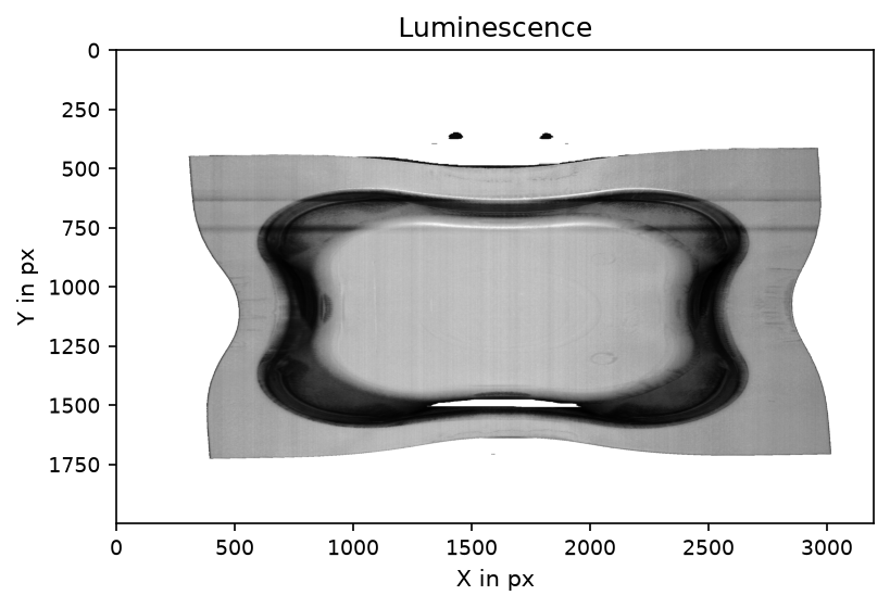
Each scan carries a second, pixel-aligned buffer: the luminescence (reflected intensity). It reads like a grayscale photo of the part and is useful for spotting surface defects, oil residue, and scan artefacts that are invisible in the height channel. Same helper, different buffer:
with rddac.open_h5(experiment_id, data_dir=DATA_DIR) as f:
    lumi10 = f['pointcloud/op10/luminescence'][:]

ax, cbar = rddac.plot_scan(lumi10, cmap='gray', title='OP10 - luminescence')
plt.show()
3. From scan to point cloud
scan_to_pointcloud converts a flat buffer into an (N, 3) array of [x_px, y_px, z_raw], dropping invalid pixels. Passing the luminescence buffer as the second argument additionally drops pixels where the intensity is zero (no reliable measurement). stride thins the grid for fast previews — stride=4 reduces the 6.4 M pixels to roughly 400 k points:
with rddac.open_h5(experiment_id, data_dir=DATA_DIR) as f:
    z10   = f['pointcloud/op10/z'][:]
    lumi  = f['pointcloud/op10/luminescence'][:]

pts = rddac.scan_to_pointcloud(z10, lumi, stride=4)
print(pts.shape, pts.dtype)
Output:
plot_point_cloud scatters the result in 3D. By default it colours by the z coordinate and random-subsamples to max_points=200_000 so matplotlib stays responsive:
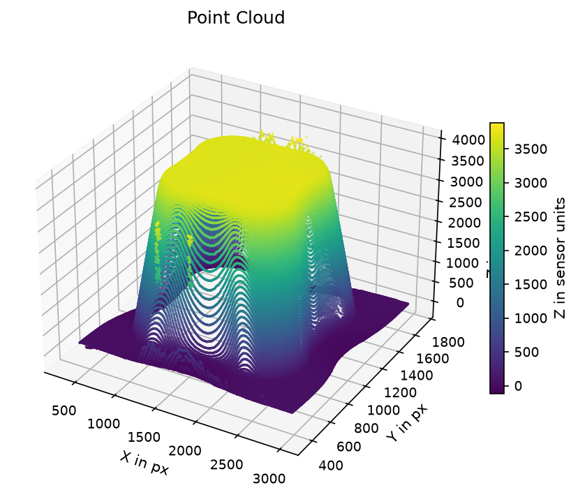
The signature mirrors ddacs.plot_point_cloud, so DDACS rendering code ports by swapping the import. values= accepts any per-point scalar — pass the luminescence of the surviving points to paint intensity onto the geometry.
4. Force signals
force/data is an (n, 8) table; the column layout lives in the group's columns attr and matches rddac.visualization.FORCE_COLUMNS. plot_force draws the selected signals against time — by default the four load cells and the total force:
with rddac.open_h5(experiment_id, data_dir=DATA_DIR) as f:
    force = f['force/data'][:]

ax = rddac.plot_force(force, title='Press signals')
plt.show()
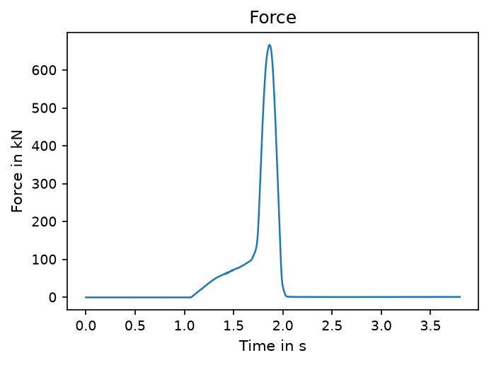
Pass signals=('punch_pos',) (or any subset of the column names) to plot other channels; plot_force raises a ValueError naming the available columns on a typo.
5. Sensor traverses
plot_traverse renders the two (n, 2) traverse tables — sheet thickness and oil film — as value over sensor position:
with rddac.open_h5(experiment_id, data_dir=DATA_DIR) as f:
    sheet = f['sheet_thickness/data'][:]
    oil   = f['oil_thickness/data'][:] if f.attrs['has_oil'] else None

ax = rddac.plot_traverse(sheet, ylabel='sheet thickness [um]', title='Sheet thickness traverse')
plt.show()
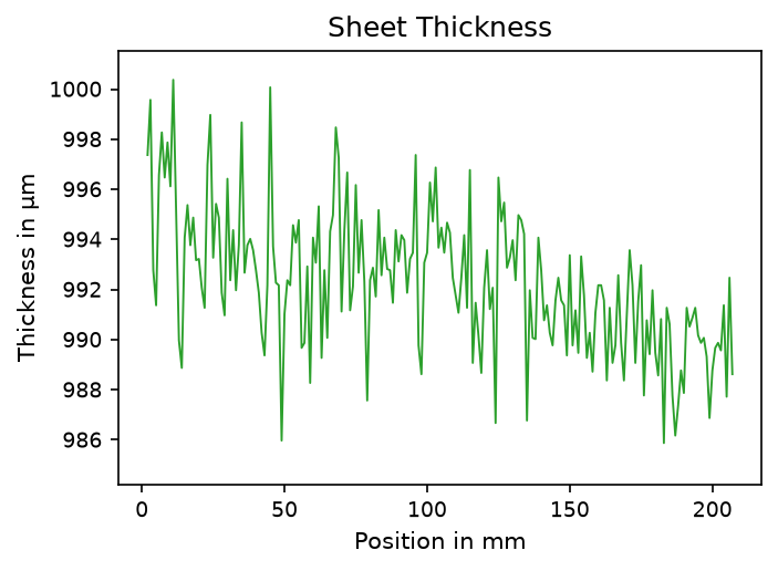
Note on the x axis: the raw sensor_position values carry the 50 mm mounting offset of the thickness sensor (positions run from 50 mm upward); the plot above shows positions with that offset removed. Subtract 50 from sheet[:, 0] to reproduce it.
if oil is not None:
    ax = rddac.plot_traverse(oil, ylabel='oil [g/m^2]', title='Oil film traverse')
    plt.show()
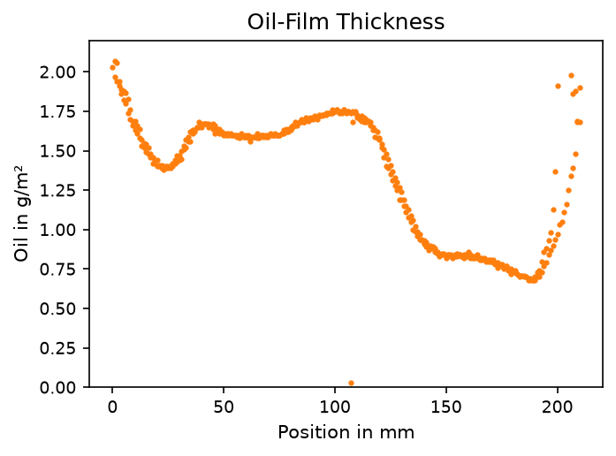
The label= argument plus a shared ax overlays multiple traverses — useful for comparing repetitions of one category:
fig, ax = plt.subplots(figsize=(10, 4))
for eid in (0, 500):        # two sample experiments
    with rddac.open_h5(eid, data_dir=DATA_DIR) as f:
        rddac.plot_traverse(f['sheet_thickness/data'][:], ax=ax,
                            ylabel='sheet thickness [um]', label=f'experiment {eid}')
plt.show()
For the full function signatures see the Visualization API reference.