Getting Started¶

This tutorial walks from installation to a first plot. It uses only the public surface that ships with v1.0.0: rddac.open_h5, rddac.inspect_h5, and the visualization helpers.

The companion notebook at notebooks/01_getting_started.ipynb reproduces every cell below; open it side by side to run as you read.

1. Install¶

pip install rddac

The PyTorch adapter is optional. Install it explicitly if a model is to be trained:

pip install rddac[torch]

For hardware specific PyTorch builds (CUDA, ROCm, MPS) see pytorch.org and install PyTorch before rddac.

Verify the install. From a Python REPL or notebook cell:

import rddac
print(rddac.__version__)

Or as a single shell command (handy on Linux servers where opening a REPL is overkill):

python3 -c "import rddac; print(rddac.__version__)"

Output:

1.0.0

2. Download the data¶

This tutorial only needs the small bundle (~174 MB) — metadata.json, process_parameters.csv and sample.zip with one experiment per category:

rddac download --small

The full dataset (~87 GB, plus the matching DDACS simulations) downloads with plain rddac download; see the CLI reference for the other options (selected files, unattended runs, extraction).

All downloads write into ./data/ and keep the zips zipped; mlcroissant reads them in place. The rest of the tutorial uses:

from pathlib import Path

DATA_DIR = Path('./data')      # repository root
# DATA_DIR = Path('../data')   # uncomment instead when running from inside notebooks/
experiment_id = 0              # one bundled sample experiment (concave, 100 kN, coarse oil)

3. Inspect one experiment¶

rddac.open_h5(experiment_id, data_dir=...) resolves the manifest, finds the right zip, reads the HDF5 member into memory and returns an h5py.File. It is read only and supports the with idiom:

with rddac.open_h5(experiment_id, data_dir=DATA_DIR) as f:
    print(list(f.keys()))

Output:

['force', 'oil_thickness', 'pointcloud', 'sheet_thickness']

rddac.inspect_h5 prints the group and dataset hierarchy of an open file or a path on disk:

with rddac.open_h5(experiment_id, data_dir=DATA_DIR) as f:
    rddac.inspect_h5(f)

Output (truncated; the full tree is in HDF5 structure):

0000.h5
├── @blankholder_force = 100
├── @geometry = concave
├── @oil_type = coarse
├── @has_oil = True
├── @has_pointcloud = True
├── force/
│   ├── @columns = ['time' 'load_cell_1' ... 'total_force']
│   ├── @units = ['s' 'kN' ... 'kN']
│   └── data  (1140, 8) float32
├── oil_thickness/
│   └── data  (421, 2) float32
├── pointcloud/
│   ├── op10/   (z + luminescence, flat (6400000,) buffers)
│   └── op20/   (z + luminescence, flat (6400000,) buffers)
└── sheet_thickness/
    └── data  (208, 2) float32

Each line that starts with @ is an HDF5 attribute. Groups end in /; datasets show their shape and dtype. Note the table groups carry their own columns and units attributes.

4. First plot¶

The next cell renders the OP10 laser scan — the formed cup after deep drawing — as a 3D point cloud. Two buffers drive the plot:

z : the raw height buffer. pointcloud/op10/z is a flat (6400000,) array stored row-major over the 2000 x 3200 pixel grid declared by the group's y_shape / x_shape attributes.
luminescence : the matching intensity buffer. Pixels where the scanner measured nothing carry 0; passing the buffer to scan_to_pointcloud drops them, so only real measurements become points.

rddac.scan_to_pointcloud turns the buffers into an (N, 3) array of [x_px, y_px, z_raw]; stride=4 keeps every fourth pixel in both axes (~400k points instead of 6.4 million — plenty for a preview). The values are raw sensor units (uncalibrated) — good enough for inspection; the mm calibration belongs to the planned preprocessing step.

import matplotlib.pyplot as plt
import rddac

with rddac.open_h5(experiment_id, data_dir=DATA_DIR) as f:
    z    = f['pointcloud/op10/z'][:]
    lumi = f['pointcloud/op10/luminescence'][:]

points = rddac.scan_to_pointcloud(z, lumi, stride=4)      # (N, 3): x_px, y_px, z_raw
ax, cbar = rddac.plot_point_cloud(points, point_size=0.4, title='OP10 - after deep drawing')
cbar.set_label('z in sensor units')
plt.show()

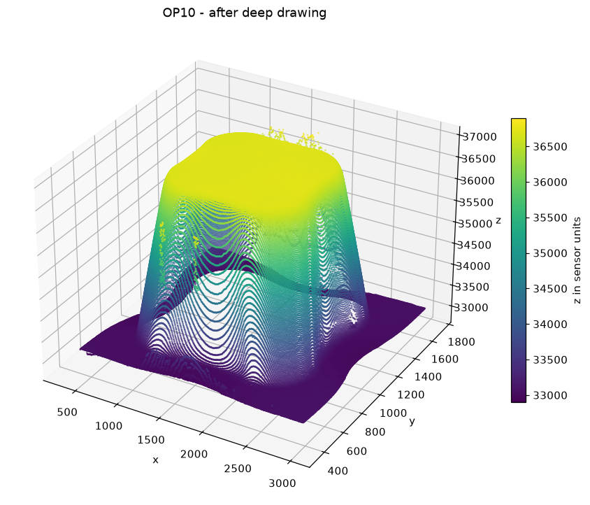
plot_point_cloud returns (ax, cbar): the matplotlib 3D axis and the colorbar. Both can be customised afterwards (e.g. ax.view_init(...) for a different camera angle, cbar.set_label(...) to change the label). By default the points are colored by their z value; pass values=... to color by anything else per point.

Where to go next¶

Build your own view introduces rddac.load, the manifest's RecordSets, and rddac.add_view for custom field selections.
PyTorch training covers RDDACDataset, multi worker DataLoader, DDP, and filtering.
Visualization covers scans, point clouds, force curves and traverses in depth.
Loose HDF5 recipe shows the CSV plus h5py.File iteration loop for users who run rddac download --extract --remove-zip.